Introduction
Package splinemixmeta provides some basic capabilities
in non-parametric meta-regression. If one has responses y,
each with a standard error, from previous analyses, and wants to regress
those against study-level explanatory variables x without
assuming linearity, splinemixmeta allows an arbitrary
smooth relationship to be estimated as a smoothing spline. It is also
possible to include other explanatory variables (assumed to have a
linear relationship to y) and random effects groupings.
Such an approach may be referred to as “non-parametric meta-analysis”,
“spline meta-regression”, “meta-splines”, or other similar terminology
mash-ups.
splinemixmeta works by bringing together features of
mgcv for building spline components and
mixmeta for estimating general mixed-effects meta-analysis
models. Specifically, the splines of mgcv can be used as
random effects components, with the penalty matrix providing a
correlation structure for spline coefficients, the unknown smoothness
parameter replaced by an unknown variance parameter, and any unpenalized
directions in the spline parameter space (e.g. spline parameters
representing a linear relationship) moved into fixed effects. The
resulting pieces are then set up as needed for a call to
mixmeta::mixmeta for estimating the model. Variance
parameters are always estimated by REML (restricted maximum
likelihood).
There are some important limits on what will work. At the moment, the
only recommended spline basis functions are bs="cr",
bs="cs", and bs="cc". These are supported
because the associated covariance matrices can be diagonalized. The
mgcv default of bs="tp" does not currently
produce good results. One can have multiple spline components, although
this is rather limited because most of the choices in mgcv
for bivariate splines are not among those supported. It is possible that
bs = "mrf" also works, but it has not been tested. See
help(splinemixmeta) for more about what is supported.
The estimation machinery is not particularly efficient and so may be notably slow for large models.
Example
Here we give a simulated example. Say we have n=50
values, with 5 values from each of 10 groups, with a sinusoidal
relationship between y and x to provide a
simple nonlinear example. The groups will be treated as random effects,
as will the spline. The simplest case would not have groups, but here we
illustrate a case that does.
Data simulation
set.seed(1)
n <- 50
num_groups <- 10
group <- rep(1:num_groups, each = 5) |> factor()
group_effects <- rnorm(length(group), 0, 0.3)
x <- runif(n, 0, 20)
coef_x <- 0.6
se <- runif(n, 0.1, 0.3)
fx <- 1.5 * sin(2 * pi * x / 12)
y <- 10 + coef_x * x + fx +
  group_effects[group] +
  fx + rnorm(n, 0, 1) + rnorm(n, 0, se)
data <- data.frame(y, x, se, group)
plot(y ~ x, data = data, col = group, pch = 19, main = "Simulated data (color = group)")
This data simulation has the following pieces:
- We have 10 groups of 5 data points each. (Since the
xvalues are all drawn independently, the groups are independent fromx.) -
xis uniformly distributed from 0 to 20. - We assume each
ywas obtained separately from a previous study, and these studies are grouped in some relevant way (e.g. from the same study region or same lab). - Fixed effects for
yinclude an intercept and linear term. - Random effects for
yinclude the group effects. - The sinusoidal term for
ywill be estimated as a spline, treated as a random effect. - Residuals are normally distributed with
sd = 1. - Measurement errors (i.e. estimation error from the previous studies
from which
ywere obtained) are normally distributed with standard deviations that are the standard errors (se) from the previous studies. These standard errors are simulated as uniformly distributed between 0.1 and 0.3 to reflect heterogeneity in the precision of the previous studies.
Estimation of a spline meta-regression model
The spline meta-regression model can be estimated like this:
library(splinemixmeta)
smm <- splinemixmeta( mgcv::s(x, bs = "cr"), y ~ x,
                      se = se, manual_fixed = TRUE,
                      data = data, random = ~ 1 | group)
The object smm will have class “splinemixmeta” and
“mixmeta”. First we can look at a summary of the model:
summary(smm)
#> Call:  mixmeta::mixmeta(formula = y ~ x, S = (se)^2, data = data, random = list(
#>     ~basisFxns_A - 1 | all, ~1 | group, ~1 | ID), bscov = c("id",
#> "unstr", "unstr"))
#>
#> Univariate extended random-effects meta-regression
#> Dimension: 1
#> Estimation method: REML
#>
#> Fixed-effects coefficients
#>              Estimate  Std. Error        z  Pr(>|z|)  95%ci.lb  95%ci.ub
#> (Intercept)   11.6246      0.3215  36.1600    0.0000   10.9945   12.2547  ***
#> x              0.4509      0.0265  17.0192    0.0000    0.3990    0.5028  ***
#> ---
#> Signif. codes:  0 '***' 0.001 '**' 0.01 '*' 0.05 '.' 0.1 ' ' 1
#>
#> Random-effects (co)variance components
#>  Formula: ~basisFxns_A - 1 | all
#>  Structure: Multiple of identity
#>               Std. Dev          Corr
#> basisFxns_A1    0.4490  basisFxns_A1  basisFxns_A2  basisFxns_A3  basisFxns_A4
#> basisFxns_A2    0.4490             0
#> basisFxns_A3    0.4490             0             0
#> basisFxns_A4    0.4490             0             0             0
#> basisFxns_A5    0.4490             0             0             0             0
#> basisFxns_A6    0.4490             0             0             0             0
#> basisFxns_A7    0.4490             0             0             0             0
#> basisFxns_A8    0.4490             0             0             0             0
#>
#> basisFxns_A1  basisFxns_A5  basisFxns_A6  basisFxns_A7
#> basisFxns_A2
#> basisFxns_A3
#> basisFxns_A4
#> basisFxns_A5
#> basisFxns_A6             0
#> basisFxns_A7             0             0
#> basisFxns_A8             0             0             0
#>
#>  Formula: ~1 | group
#>  Structure: General positive-definite
#>   Std. Dev
#>     0.4097
#>
#>  Formula: ~1 | ID
#>  Structure: General positive-definite
#>   Std. Dev
#>     0.8835
#>
#> Univariate Cochran Q-test for residual heterogeneity:
#> Q = 6358.8466 (df = 48), p-value = 0.0000
#> I-square statistic = 99.2%
#>
#> 50 units, 1 outcome, 50 observations, 2 fixed and 3 random-effects parameters
#>   logLik       AIC       BIC
#> -76.3152  162.6304  171.9864
The spline terms are labeled as basisFxns_A. Further
splines would be basixFxns_B, etc.
Two factors have been introduced. One is called all,
which has a single level for every row of the data, which facilitates
use of mixmeta::mixmeta. The other is called
ID, which has a unique value for each row. In
meta-regression, it can be tempting to think that the standard errors
associated with y values serve as the only source of
residual variation, but that is not typically the case. If each
y came from a large sample size in the previous studies,
the standard errors would be small, but we would still expect
study-level variation around any regression line because the world is
noisy. That study-level variation, i.e. additional residual variation,
is set up as a random effect with one level for each y.
By using y ~ x, we included a linear term for
x directly (manually), and thus we needed to set
manual_fixed = TRUE. Otherwise splinemixmeta
would have obtained a linear term from the spline setup and included it
in the model, and we don’t want it duplicated. (Such a linear term, or
more generally unpenalized dimensions of the spline coefficients, will
always be removed from the smooth term when it is converted into the
format of a random effect.) In the summary output, we see
the full covariance matrix from the spline random effect, which is the
vector of spline coefficients. This is shown as the standard deviation
for each component (all the same) and their correlations (all 0),
reflecting a covariance matrix that is a constant times an identity
matrix. It has this structure because the random effects structure from
the spline basis functions and penalty matrix are rotated in order to
work with a diagonal covariance matrix.
Finally we see the estimated standard deviation between groups and
the estimated residual standard deviation, shown as the
~1 | ID term.
(If the default names all or ID are already
used in the data set, splinemixmeta will choose different
names.)
Predictions
Predictions can be obtained at multiple levels of the random effects.
The predict function for splinemixmeta objects
simplifies this by allowing the choices of including any spline terms
(default TRUE), other random effects (default
FALSE but possibly of interest) and residuals (default
FALSE and typically not of interest). Predictions will come
with columns for standard errors and variances (squared standard
errors). The machinery for predictions is modified from
mixmeta::blup(), where “blup” means “best linear unbiased
predictor”, a standard term in linear mixed effects modeling. Hence the
column of predictions returned by predict is labeled
“blup”. The blups come from the conditional distribution of
random effects, given the data and estimated variance parameters.
Following mixmeta::blup, predictions can be of type
“outcome”, in which case variance from fixed effects terms is included
in the prediction variance (and standard errors), or “residual”, in
which case only variance from random effects is included. The default is
“outcome”. See help(predict.splinemixmeta) for details. Any
further fine-grained control (such as including one spline but not
another), can be done by calling splinemixmeta::blup()
directly.
Here are two versions of predictions:
pred_spline_only <- predict(smm, include_smooths = TRUE, include_REs = FALSE, include_residuals = FALSE, type = "outcome")
pred_spline_and_groups <- predict(smm, include_smooths = TRUE, include_REs = TRUE, include_residuals = FALSE, type = "outcome")
# look at both together
head(cbind(pred_spline_only, pred_spline_and_groups))
#>       blup        se      vcov     blup        se      vcov
#> 1 19.01618 0.3506960 0.1229877 18.74330 0.4357595 0.1898863
#> 2 12.91852 0.5107873 0.2609037 12.64564 0.5430035 0.2948528
#> 3 14.19637 0.4093650 0.1675797 13.92349 0.4706131 0.2214767
#> 4 19.25014 0.5170299 0.2673199 18.97727 0.5765052 0.3323583
#> 5 18.31537 0.3538785 0.1252300 18.04249 0.4386054 0.1923747
#> 6 14.81859 0.3818512 0.1458104 15.43221 0.4673896 0.2184530
# look at only fixed effect, which could be done with `predict`
# but here we illustrate a direct call to `blup`
blup(smm, level=0, vcov = TRUE, se = TRUE) |> head()
#>       blup        se       vcov
#> 1 17.52867 0.2001708 0.04006835
#> 2 14.80961 0.1982734 0.03931235
#> 3 14.06172 0.2192172 0.04805620
#> 4 20.57627 0.3187314 0.10158973
#> 5 17.33722 0.1958174 0.03834447
#> 6 13.54724 0.2373041 0.05631323
Figures
splinemixmeta provides a basic capability for figures,
for which the suggested package ggplot2 is needed.
plot(smm, ylab = "y", title = "Spline meta-regression fit")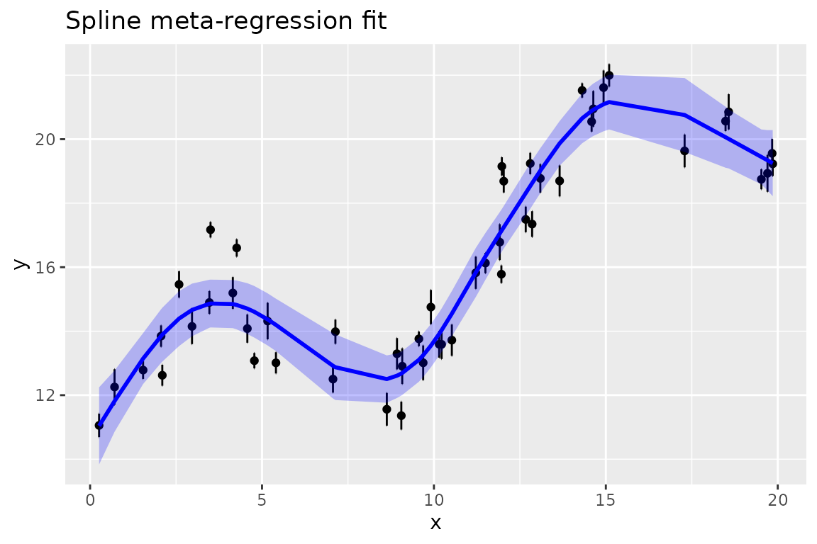
In this figure, the y values are shown with approximate
95% confidence intervals calculated as +/- 2 standard errors, from the
standard errors that were input as the se argument to
splinemixmeta. The fitted line by default includes fixed
effects and spline terms (blups), with a 95% confidence envelope.